Ensemble Deep learning model using panoramic radiographs and clinical variables for osteoporosis disease detection
T Ramesh1, V Santhi1
1School of Computer Science and Engineering, Vellore Institute of Technology, Vellore, 632014, Tamil Nadu, India
Corresponding Author:T Ramesh (e-mail: t.ramesh2014@vit.ac.in)
DOI: https://doi.org/10.59461/ijdiic.v4i1.158
Article history: Received November 07, 2024, Revised December 19, 2024, Accepted January 01, 2025
ABSTRACT
Worldwide, a large number of people suffer from the bone disease osteoporosis. Accurate diagnosis and classification are essential for managing and preventing many disorders. In order to classify bone density images into two categories—normal and osteoporotic—this study suggests a hybrid model that combines a multiclass Support Vector Machine (MSVM) with a Deep Convolutional Neural Network (DCNN). The bone density pictures are subjected to feature extraction by the DCNN, and the information is then classified into two categories using the MSVM. The National Health and Nutrition Examination Survey (NHANES) database's dataset of bone density photos was used to train and evaluate the suggested hybrid model. According to the results, the ensemble model performs better than the most advanced methods available today in terms of F1 score, sensitivity, accuracy, and specificity. According to our research, osteoporosis may be efficiently classified by the DCNN and MSVM ensemble model, which can help with the diagnosis and treatment of various bone disorders. The proposed model gives better performance in terms of accuracy of 0.8913 and specificity of 0.9123 when compared to other models. Thus, a deep-learning diagnostic network applied to lumbar spine radiographs could facilitate screening for osteoporosis.
This is an open access article under the CC BY-SA license.

Keywords: Osteoporosis, Deep Convolutional Neural Network, Deep learning, Machine Learning, Image processing
1. INTRODUCTION
The disorder known as osteoporosis weakens bones, leaving them brittle and easily broken. This results from an excessive loss of bone mass, insufficient production of bone mass, or both. While osteoporosis can damage any bone, the spine, hip, and wrist are the most commonly affected, and it usually proceeds slowly. Because there are no symptoms until a fracture happens, it is frequently called the "silent disease". Males and females can equally suffer from osteoporosis disease, but women are more inclined to have it, particularly after menopause. A family history of osteoporosis, smoking, heavy alcohol use, being underweight, leading a sedentary lifestyle, and using specific drugs or medical conditions are risk factors. Regular exercise, a diet high in calcium and vitamin D, and abstaining from smoking and excessive alcohol are just a few examples of lifestyle modifications frequently included in treatment. Medication may be recommended to reduce bone loss or improve bone density.
In September 2021, a bone mineral density (BMD) test will be the accepted approach for diagnosing osteoporosis. A T-score is generated by comparing the results of bone mineral density (BMD) tests—which commonly evaluate the concentration of minerals in the hip, spine, and wrist—to the average BMD of a young adult who is healthy and of the same sex and race. A T-score of -1.0 or higher shows normal bone density, a T-score of -1.0 to -2.5 indicates poor bone density, and a T-score of -2.5 or lower suggests osteoporosis (very low bone density), according to the World Health Organization (WHO). However, the T-score is just one factor in assessing fracture risk due to osteoporosis. Other factors such as age, sex, medical history, family history, and lifestyle choices (e.g., smoking, alcohol use, physical activity) also contribute to the overall risk. It's important to discuss your personal risk factors and the appropriate screening schedule with your healthcare provider. New research or updated clinical guidelines may eventually lead to changes in the standards for identifying osteoporosis disease.
Deep learning algorithms can be employed to classify osteoporosis disease, a condition that affects bone health. Low bone density and bone tissue degeneration are hallmarks of osteoporosis disease, which leads to brittle bones that are more likely to break. Deep learning models are highly effective tools for diagnosing medical conditions like osteoporosis. These models use neural networks to recognize patterns in medical images, such as bone density scans, and can accurately predict whether a patient has osteoporosis or normal bone density. To develop a deep learning model for classifying osteoporosis disease, medical images from bone density scans can be used as input data. The model can be trained on a large dataset of bone density scans, with labels indicating whether each scan shows osteoporosis or normal bone density. By analyzing these scans, the model can learn to identify patterns and features that distinguish between these classifications. Once trained, the model can be used to classify new bone density scans as either showing osteoporosis or normal bone density. This can help medical professionals accurately diagnose patients and create treatment regimens that work for them.
The new gold standard for diagnosing osteoporosis is central dual-energy X-ray absorptiometry (DXA) [1]. However, the use of DXA is limited by accessibility issues, often requiring patients to visit specialized centres [2]. Reduced financial incentives and a lack of knowledge about the test are two more obstacles to DXA screening. Therefore, the percentage of Chinese women over 50 who have had a DXA test is just 4.3% in rural regions, the number is as low as 1.9% [3]. About half of female Medicare enrollees in the United States do not get tested, and screening rates are only about 10%, even in high-risk areas [2]. DXA imaging primarily assesses the presence of bones and muscles, which are often affected by fat [4]. Furthermore, DXA is only able to partially account for the size, form, and microstructure of bones due to its use of a two-dimensional projection approach. As a result, osteoporosis may not be accurately diagnosed, and DXA remains underutilized. To change these conditions, safe and reasonably priced alternatives are required. In hospitals worldwide, conventional X-ray technology is commonly available and can yield data regarding bone mineral density (BMD). Retrospective analysis of BMD data from lumbar spine X-ray pictures obtained for other purposes could be done at no additional cost or radiation exposure to patients. In general, this could lead to a rise in the number of people tested for osteoporosis. However, visually assessing BMD on lumbar spine X-ray images can be challenging.
Deep Convolutional Neural Networks have been extensively used in medical imaging, including the classification of osteoporosis disease based on bone density scans. To train a DCNN model for osteoporosis classification, a large dataset of bone density scans with corresponding T-scores is necessary. The model is trained to recognize features in the scans associated with low bone density and specific T-score categories (normal or osteoporosis). Many convolutional layers, pooling layers, and fully connected layers are the next layers seen in a typical DCNN model. The pooling layers assist in reducing the dimensionality of the data, while the convolutional layers utilize the bone density scans to identify features such as patterns of bone loss or areas with decreased density. Finally, the completely connected layers carry out the classification. Once trained, the DCNN model can be used to predict the T-score category of a new bone density scan by processing the scan through the model and obtaining the predicted category.
Deep Convolutional Neural Networks (DCNNs), a kind of deep learning system, have advanced computer vision significantly in recent years. Through several levels of abstraction, deep learning approaches gradually create feature representations by processing raw image pixels and associating them with appropriate labels from medical imaging data. With continuous advancements in DCNN architecture and the growing power of hardware, DCNNs have achieved human-level performance in tasks such as face recognition, video game playing, and natural language processing [5]. The potential advantages of DCNNs have also been demonstrated in numerous preliminary studies across various medical imaging fields, including radiology [6], pathology [7], dermatology [8], and ophthalmology [9].
2. RELATED WORKS
There are several challenges associated with using machine learning methods to detect osteoporosis, including the fact that the process is typically divided into two phases: the feature selection phase and the classification phase. However, as demonstrated in further testing, the suggested deep learning-based method not only automates feature extraction and categorization but also exhibits superior classification accuracy when assessed using both T-scores and Z-scores. Additional advantages of this approach include reduced classification time and lower error rates.
Various deep learning algorithms contribute to improving learning efficiency by expanding the range of potential applications and accelerating computational processes. However, the extended training times of deep learning models remain a significant challenge for researchers. Increasing the number of model parameters or the amount of training data can also greatly improve classification accuracy [10]. To address these challenges, the literature has introduced several state-of-the-art techniques to speed up deep learning processing. Deep learning frameworks integrate modular algorithms with infrastructure support, distribution strategies, and optimization techniques. These frameworks are designed to accelerate system-level development and research while simplifying the implementation process. This section highlights some of these notable frameworks and methods.
A Convolutional Neural Network (CNN) was developed to classify osteoporotic and normal vertebral bodies using lateral radiographs, achieving an accuracy of 92.2% in distinguishing between the two [17]. Another study utilized a deep learning model based on a modified VGG-16 network to detect and classify osteoporotic vertebral fractures on CT images. This model reached an accuracy of 94.2% in detecting osteoporotic fractures and 92.7% in classifying [10]. The use of deep learning algorithms in the automated diagnosis of osteoporosis is summarized in a review article [11], discussing various models such as CNNs, Recurrent Neural Networks (RNNs), and hybrid models. A systematic review assessed the performance of deep learning models in detecting osteoporotic fractures in CT images, finding that these models achieved high accuracy and could potentially be used for automated fracture detection [12]. Another study evaluated the effectiveness of machine learning models in predicting osteoporosis, showing that these models also achieved high accuracy and could serve as tools for early diagnosis and prevention [13][25].
Numerous studies have explored the use of Deep Convolutional Neural Networks and Multiple Support Vector Machines for classifying medical datasets. Here are some relevant works: DCNN has been employed for the classification of medical images, achieving state-of-the-art performance across various datasets, including retinal fundus images, mammography images, and brain MRI scans [14]. MSVM has been used to classify breast cancer histopathological images using local binary patterns and multiple kernel learning [15], with results showing that MSVM achieved high accuracy and outperformed other classification methods. A comparison of DCNN and MSVM for breast cancer histology image classification revealed that DCNN had superior classification accuracy. Another study combined DCNN and MSVM for lung cancer screening using CT images, successfully detecting lung nodules with high accuracy [16]. Additionally, research on classifying brain tumour MRI images found that DCNN outperformed MSVM in terms of accuracy. These studies highlight the potential of DCNN and MSVM in the classification and identification of medical images across various fields, including breast cancer, lung cancer, and brain tumours.
Model parallelism, in contrast, distributes the training process across multiple graphics processing units (GPUs). In a basic model-parallel approach, each GPU handles a portion of the model's processing. For example, in a system with two GPUs, one might be used to compute each of the LSTM layers if the model includes two, thereby speeding up overall computation. This approach enables the training and prediction of large-scale deep neural networks [17]. For instance, a COTS HPC system was employed to train a neural network with over 11 billion parameters, requiring more than 82GB of memory. Model-parallel methods are crucial when fitting a large model onto a single processor is challenging, necessitating the division of the model [18]. Since each node in a model can only compute part of the results, synchronization is required to gather the complete set of results [19]. However, because each node must synchronize gradient or attribute data at each update step, a model-parallel strategy incurs higher synchronization and communication costs than a data-parallel strategy, leading to scalability issues. Google proposed a deep reinforcement learning-based solution for autonomous device placement to optimize model partitioning and placement strategies [20]. This approach claims to boost performance by 60% compared to relying solely on human experts by combining processes based on their embedded representation. Due to the accurate detection of bone deterioration in femoral data, as indicated by BMD values [21], osteoporosis is recognized as a condition where bone breakdown exceeds bone synthesis, resulting in porous bones. Although several studies have focused on diagnosing osteoporosis, significant knowledge gaps remain due to the widespread nature of the condition [22]. Most studies found in the literature used basic datasets to support hypotheses proposed by researchers investigating the identification of osteoporosis [23].
The study using the classifier demonstrates that sequentially trained Deep Convolutional Neural Networks (DCNN) can be employed to classify osteoporosis. The objective of the DNN optimization method is to identify the network parameters that minimize the loss function. Section 3 discusses additional datasets and the primary implementation techniques.
3. MATERIALS AND METHODS
The methods section will provide a detailed description of the materials used in the study, including how they were prepared, along with an explanation of the research methodology employed.
3.1. Osteoporosis Dataset
This study compares the outcomes to DXA-defined BMD measures to assess the viability and efficacy of diagnosing osteoporosis disease in postmenopausal women using DCNN projections based on lumbar spine X-ray images obtained for various clinical objectives [27]. Deep learning could serve as a practical and cost-effective supplement to DXA screening, particularly in medical centres where DXA equipment is limited. The sample data, along with attributes and descriptions, are shown in Table 1.
Table 1. Sample Data with its Attributes and its Description
Age |
Height (cm) |
Weight (kg) |
BMI |
C.Width (mm) |
C.FD |
Tr. thick (mm) |
Tr. FD |
Tr. Numb |
Tr. separa (mm) |
62 |
153 |
55.15 |
23.4 |
1.73 |
0.87 |
0.13 |
0.22 |
2.14 |
0.71 |
60 |
182 |
76.82 |
23.13 |
3.76 |
0.54 |
0.22 |
0.15 |
2.05 |
0.5 |
72 |
152 |
68.94 |
29.75 |
2.32 |
0.87 |
0.2 |
0.3 |
2.18 |
0.61 |
65 |
183 |
72.85 |
21.59 |
4.19 |
0.38 |
0.18 |
0.44 |
2.44 |
0.53 |
80 |
152 |
80.2 |
34.68 |
3.08 |
0.59 |
0.13 |
0.17 |
2.38 |
0.26 |
60 |
150 |
75.11 |
33.06 |
3.9 |
0.46 |
0.23 |
0.33 |
2.14 |
0.55 |
65 |
177 |
76.99 |
24.33 |
4.44 |
0.62 |
0.09 |
0.11 |
2.17 |
0.28 |
57 |
189 |
74.32 |
20.61 |
4.02 |
0.4 |
0.1 |
0.59 |
1.39 |
0.52 |
53 |
185 |
70.45 |
20.39 |
4.1 |
0.8 |
0.15 |
0.18 |
1.33 |
0.67 |
89 |
173 |
88.59 |
29.59 |
2.72 |
0.81 |
0.1 |
0.27 |
1.94 |
0.66 |
53 |
186 |
50.61 |
14.52 |
3.16 |
0.87 |
0.24 |
0.11 |
1.22 |
0.73 |
74 |
150 |
79.92 |
35.42 |
2.26 |
0.39 |
0.22 |
0.36 |
1.83 |
0.28 |
52 |
189 |
78.28 |
21.91 |
2.09 |
0.67 |
0.12 |
0.6 |
1.47 |
0.72 |
81 |
169 |
85.81 |
29.82 |
3.02 |
0.58 |
0.18 |
0.34 |
1.65 |
0.45 |
Bone mineral density, fractures, falls, and other clinical parameters in older men are all being gathered for the Osteoporotic Fractures in Men Study (MrOS), a longitudinal study. Through the Biologic Specimen and Data Repository Information Coordinating Center (BioLINCC) of the National Institutes of Health, this dataset is available to the public. A cross-sectional study called the National Health and Dietary Examination Survey (NHANES) collects information on a range of dietary and health-related topics, including bone health. The general public can access it through the Centers for Disease Control and Prevention (CDC). The Study of Osteoporotic Fractures (SOF) is another longitudinal study that focuses on bone mineral density, fractures, and other clinical measures in older women, with data available through the National Institute on Aging (NIA). The National Heart, Lung, and Blood Institute (NHLBI) offers information about the Framingham Osteoporosis Study, a longitudinal investigation that gathers data on bone mineral density, fractures, and other clinical variables in older men and women. Additionally, the UK Biobank is a large-scale prospective study that gathers data on various health-related factors, including bone health and is accessible to researchers who apply for and receive approval from the UK Biobank Access Committee. These datasets are valuable resources for osteoporosis research and have been utilized in studies to develop and validate diagnostic and predictive models.
3.2. Proposed Architecture
Bone mineral density (BMD) measurements are a frequent method used in the building of a classification system for osteoporosis disease. As a measure of bone strength, BMD measures the amount of minerals present in bone tissue. A potential design for an osteoporosis classification system based on BMD might include the following criteria:
- Normal BMD: Within one standard deviation (SD) of the average BMD for a reference group of young adults.
- Osteopenia: BMD that is between one and 2.5 standard deviations below the mean BMD of the young adult reference sample.
- Osteoporosis: BMD greater than 2.5 SD lower than the reference group's mean BMD of young adults.
Additionally, the following subcategories could be part of the classification system: A BMD that is more than 2.5 SD lower than the mean BMD for the reference group of young adults, and one or more fragility fractures are indicators of severe osteoporosis. In addition to one or more variables that raise the risk of fracture, osteoporosis is defined by a BMD that is more than 2.5 SD lower than the mean BMD for young people. A bone fracture history or other medical factors that raise the risk of fracture are combined with a BMD that is one to 2.5 SD lower than the reference group's mean BMD to be classified as high fracture risk. Low bone mass is characterized by a BMD between 1 and 2.5 SD below the mean BMD for young adults without a history of fractures or other medical risk factors for fractures. The flow chart of patient inclusion to enhance the classification of osteoporosis disease is shown in Figure 1. This classification system helps guide clinical decision-making, but it's important to remember that BMD is not the sole determinant of fracture risk; other clinical risk factors should also be considered when making treatment decisions.
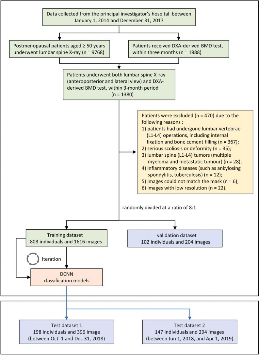
Figure 1. Flowchart of patient inclusion in a multi-centre study. This network architecture uses direct layer-to-layer connections to bypass layers, improve feature transmission, and enhance data flow integration [30].
3.2.1. X-rays of the lumbar spine
Lumbar spine X-rays are not the most reliable way to detect osteoporosis disease, as these conditions primarily affect bone density, which standard X-rays cannot detect [24]. However, lumbar spine X-rays can help identify fractures or structural changes in the bone that may indicate osteoporosis. For instance, individuals with osteoporosis might have compression fractures in their vertebrae visible on X-rays. X-rays can also be used alongside other diagnostic tests, such as bone density scans, to aid in diagnosing osteoporosis. Compared to X-rays, bone density scans, such as dual-energy X-ray absorptiometry (DXA), are more accurate and sensitive to identifying changes in bone density [26]. Early detection and treatment of osteoporosis are crucial for preventing fractures and other complications.
The two channels intended to examine lateral (LAT) or anterior-posterior (AP) lumbar vertebra pictures make up the recently established CNN classification model. The basic structure of both channels is the same as it was designed to be. DenseNet, a feed-forward network where every layer is connected to all subsequent layers, was utilized to extract features. This network architecture incorporates direct connections between each layer and the layer below it, which helps bypass connections, enhance feature transmission, and facilitate data flow integration. Each layer receives the image features from all preceding layers as input and passes its generated features to the subsequent layers. This design greatly minimizes the data processing needed, solves the vanishing-gradient issue, improves feature transmission, and encourages feature reuse., as illustrated in Figure 2.
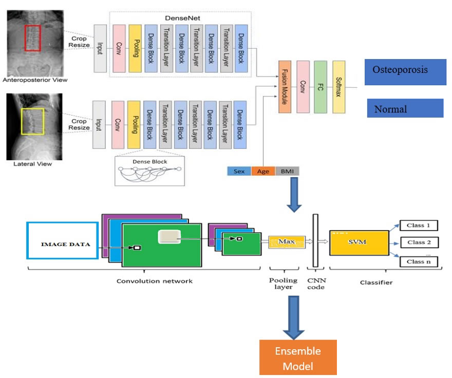
Figure 2. Architecture for the proposed model
We developed a 3-class CNN model to categorize images based on AP, LAT, or AP+LAT views, addressing the three-category classification task. Each scenario utilized a single network with two channels. To evaluate the effectiveness of the classification models, we randomly divided a total of 5,652 participants into training and validation sets in an 8:1 ratio. Furthermore, as separate test cohorts from the training cohorts, 600 patients from a different subdistrict and 600 participants from a second partner institution were involved. The models were developed using the training cohort; hyperparameters and the ideal model were chosen using the validation cohort, and the models' correctness was assessed using a test cohort. Patients were categorized into groups according to their osteoporosis levels and normal bone density using the proposed model. In order to determine whether adding clinical parameters (gender, age, and BMI) to the picture data could improve the CNN model's performance.
3.2.2. Statistic evaluation
Deep Convolutional Neural Networks (DCNN) and Multiclass Support Vector Machines are integrated into this hybrid data model. (MSVM) can be structured as follows:
- Data Preprocessing: The input data is preprocessed to extract pertinent features for both the DCNN and MSVM models. This step may include normalization, data augmentation, and feature selection techniques.
- DCNN Model: The preprocessed data is input into the DCNN model to extract high-level features. The DCNN learns representations that the MSVM model will employ through extensive dataset training. The DCNN’s output is then flattened and provided as input to the MSVM model.
- MSVM Model: The flattened output from the DCNN model is fed into the MSVM model, which is trained to classify the data into multiple categories. The MSVM model can be fine-tuned using a smaller dataset to enhance its performance.
- Ensemble: The results from both the DCNN and MSVM models are combined using an ensemble method. This could involve averaging the probabilities from both models or using a weighted average to prioritize one model over the other.
- Evaluation: Common criteria, including accuracy, precision, recall, and F1 score, are used to evaluate the efficacy of the hybrid model. The performance of the hybrid model may also be compared with other advanced models to evaluate its efficacy.
3.2.3. DCNN Model Architecture
A Deep Convolutional Neural Network (DCNN) can be utilized to detect features in the input image. The architecture of the DCNN model may be structured as follows:
Input Layer: The preprocessed image is fed into the input layer of the DCNN model.
Convolutional Layers: These layers process the image via several filters in order to retrieve relevant information.
Pooling Layers: The feature maps produced by the convolutional layers are less dimensional through pooling layers.
Activation Function: Non-linearity is introduced by applying an activation function to the convolutional and pooling layers' outputs.
Fully Connected Layers: Classifying an input image is done by these layers using the features that have been extracted.
3.2.4. MSVM Model Architecture
The Multiclass Support Vector Machine (MSVM) model is intended to classify the input image into various categories. Its architecture is structured as follows:
Input Layer: The DCNN model's flattened output is fed into this layer.
Support Vector Machine: The SVM component learns to classify the input image into multiple classes based on the features extracted by the DCNN model.
Ensemble Architecture: The results from both the DCNN and MSVM models are combined using an ensemble technique. This may involve averaging the probabilities from each model or applying a weighted average to emphasize one model over the other.
The DCNN and MSVM model offers a robust framework for image classification tasks. By leveraging the strengths of both models, this hybrid approach can enhance the accuracy and reliability of the classification process. The architecture of the model can be tailored and fine-tuned based on the specific dataset and task requirements.
Algorithm
Here's a pseudo-code algorithm for DCNN and MSVM models -:
DCNN Algorithm:
Input: Preprocessed image data
Output: Features extracted by the DCNN model
- Load pre-trained DCNN model
- For each image in the dataset:
a. Feed the image through the DCNN model
b. Flatten the output of the DCNN model
c. Store the flattened output as features for the image
- Return the extracted features for all images
MSVM Algorithm:
Input: Features extracted by the DCNN model
Output: Classification results for the input data
- Train the MSVM model using the extracted features and the corresponding labels
- For each image in the test set:
a. Feed the flattened output from the DCNN model as input to the MSVM model
b. Use the MSVM model to classify the image into one of the predefined classes
c. Store the classification result for the image
- Return the classification results for all images in the test set
Note: The aforementioned approach relies on the assumption that MSVM models is a multiclass SVM that can divide the input data into many classes. If the SVM model is a classification method, it may be trained to divide the input data into several categories using a one-vs-all method.
DCNN A kind of neural network frequently employed in image identification applications is the (Deep Convolutional Neural Network). The basic equation for a convolutional layer in a DCNN as shown in equation (1).

Where w is the weight matrix, b is the bias term, y (i, j, k) is the output at position (i, j) in channel k, and x (p, q, r) is the input at position (p, q) in channel r. Any nonlinear function, such as the Rectified Linear Unit (ReLU), can be used as the activation function.
A well-liked machine learning technique called SVM is utilized for regression and classification applications. The basic equation for a linear SVM is shown in equation (2).

Where w is the weight vector, b is the bias term, and sign is the sign function that returns +1 for positive values and -1 for negative values. y(x) is the projected class label for input x. By minimizing a loss function while keeping in mind a constraint that maintains a margin of separation between the classes, the weight vector and bias term are learned during training.
One-vs-all (OVA) or one-vs-one (OVO) techniques can be applied to the multiclass category. Every class in OVA has its own SVM trained for it, and the class that produces the greatest SVM output is chosen as the prediction during testing. For every pair of classes in OVO, a single SVM is trained, and during testing, the class that receives the most votes from the SVMs is chosen as the forecast. A hybrid model that combines a Deep Convolutional Neural Network (DCNN) and a maximum margin support vector machine (MSVM) can be formulated as follows:
Let x be the input data, y be the ground truth label, and f(x) be the output of the DCNN. The output of the hybrid model can be represented in equation (3).

Where w and b are the weight vector and bias term learned by the MSVM. The sign function is used to map the output to a binary prediction. To train the hybrid model, we first pre-train the DCNN on a large dataset using unsupervised learning, such as the autoencoder or denoising autoencoder. Then, we fine-tune the DCNN on the task-specific dataset using supervised learning, such as the softmax regression or multi-task learning. Finally, we use the fine-tuned DCNN as a feature extractor and train the MSVM on the extracted features to obtain the weight vector and bias term. The hybrid model can achieve better performance than either the DCNN or the MSVM alone by leveraging the strengths of both models: the DCNN can learn high-level features from raw data, while the MSVM can learn a discriminative decision boundary between the classes.
4. RESULTS AND DISCUSSION
The outcomes of the CNNs for LS x-ray data used to detect osteoporosis are displayed in Table 1. The model was based on the Anterior-Posterior + Lateral channel for diagnosing osteoporosis and performed best among the validation cohort and the two test cohorts, with just an AUC range from 0.894 to 0.993, a specificity range from 79.98% t- 88.45%, a specificity range from 82.54% - 86.63%, as well as a negative prediction accuracy range from 90.08% - 91.15%. evaluating the ROC curves of CNN models with individual and coupled image algorithms (Figure 3). The percentage of false-positive, true-positive, true-negative, & false-negative outcomes is provided by the classification confusion metrics of approaches that rely on the AP+LAT channel, which are displayed in Table 2.
Table 2. Outcome CNN model for detecting osteoporosis based on metrics
Datasets |
Image projection |
AUC (95% CI) |
Sensitivity (%) |
Specificity (%) |
PPV (%) |
NPV (%) |
Training |
AP |
0.995 |
99.95 |
99.93 |
99.89 |
99.96 |
LAT |
0.995 |
99.95 |
99.96 |
99.95 |
99.96 |
|
AP and LAT |
0.965 |
89.98 |
90.02 |
81.64 |
94.81 |
|
Validation |
AP |
0.905 |
82.15 |
85.65 |
76.04 |
89.65 |
LAT |
0.888 |
75.46 |
85.65 |
74.46 |
86.27 |
|
AP and LAT |
0.938 |
84.83 |
86.64 |
77.86 |
91.16 |
|
Test cohort 1 |
AP |
0.889 |
81.52 |
81.77 |
69.35 |
89.74 |
LAT |
0.912 |
80.08 |
86.08 |
74.44 |
89.52 |
|
AP and LAT |
0.932 |
82.93 |
85.84 |
74.78 |
90.85 |
|
Test cohort 2 |
AP |
0.891 |
80.47 |
81.11 |
68.14 |
89.20 |
LAT |
0.873 |
73.80 |
81.35 |
66.53 |
86.09 |
|
AP and LAT |
0.908 |
81.91 |
82.53 |
70.21 |
90.09 |

Figure 3. Metrics Analysis for Sensitivity and Specificity
Table 3. Confusion matrices Anterior-posterior and Lateral
Valid Process |
Execution 1 |
Execution 2 |
||||
Osteoporosis |
Normal |
Osteoporosis |
Normal |
Osteoporosis |
Normal |
|
Osteoporosis |
189 |
1 |
169 |
2 |
186 |
1 |
Normal |
5 |
98 |
1 |
124 |
23 |
135 |
Table 1 demonstrates the dataset's partitioning and the final distributions of the test, validation, and training sets' individuals, radiographs, and vertebral bodies. The number of SQ vertebral bodies at each anatomic level of the spine is shown in Figure 3. The information was collected from the multinational MrOS study, which began in 2000. A backup plan is a smart idea in the event that something goes wrong. We are now creating more data, such as regional data with radiography, to use more contemporary methods. These data have a variety of applications. to assess the generalization of the model or even to create a better model, As shown in Table 3.
Only male participants from six healthcare facilities in the US were intended for the MrOS trial. To be sure that this approach can be used on women and people throughout the world, more testing is necessary. Further statistics with female participants or foreign content are presently being developed in order to examine the generalization of the model & train a more trustworthy model, as per Figure 4. According to several studies, the General SQ parameters have limitations for measuring OCFs [28] [29]. As per the Genant SQ criteria, subtle anterior wedge-ing correlates with a range of signs which could be misinterpreted as slightly OCF. Other OCF classification strategies, such as the improved algorithm-based qualitative method [31], are going to be employed in future research. 4.2 Comparison based on customized sequential model, proposed model with respect to other algorithms shown in Figure 5. The study may have some other drawbacks as well [32].
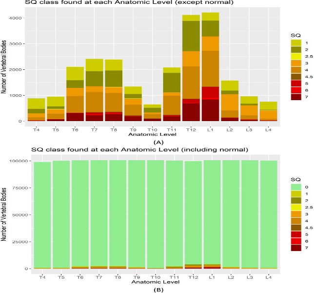
Figure 4. Number of SQ vertebral bodies at each anatomic level of the spine
Table 4. Comparison of Various Algorithms with different Metrics
Accuracy |
Precision |
Recall |
Specificity |
NPV |
F1 Score |
AUC Score |
|
ResNet18 |
0.7877 |
0.8653 |
0.7257 |
0.8626 |
0.7214 |
0.7896 |
0.9088 |
ResNet34 |
0.8406 |
0.8794 |
0.8227 |
0.8626 |
0.7 |
0.86 |
0.9204 |
GoogleNet |
0.8406 |
0.8928 |
0.8066 |
0.8823 |
0.7896 |
0.8476 |
0.9063 |
EfficientNet b3 |
0.8406 |
0.8928 |
0.8066 |
0.8823 |
0.7896 |
0.8476 |
0.9088 |
EfficientNet b4 |
0.8054 |
0.804 |
0.8547 |
0.7452 |
0.8086 |
0.8282 |
0.8787 |
Customized sequential model |
0.8791 |
0.9176 |
0.8527 |
0.9056 |
0.8367 |
0.8766 |
0.9466 |
Ensemble Model |
0.8913 |
0.9456 |
0.8711 |
0.9123 |
0.8389 |
0.8833 |
0.9513 |
DCNN |
0.7923 |
0.7533 |
0.812 |
0.745 |
0.8085 |
0.8281 |
0.8786 |
MSVM |
0.7811 |
0.7654 |
0.6258 |
0.7627 |
0.6213 |
0.6895 |
0.8089 |
First, there may have been selection bias because of the retroactive inclusion of participants who had matched LS radiographs and DXA tests. Moreover, the impact of cortical, hyperosteogeny, and arteriosclerosis sclerosis on the estimation of BMD could not be ruled out by DXA testing (11), which can cause an underestimate of real bone density loss. Similarly, how aortic sclerosis, gastrointestinal problems, and osteophytic spurs can all impact the proposed technique and cause BMD values to be overestimated, as shown in Figure 5. Finally, all ROIs were drawn by hand, which took some time but resulted in rather accurate results. Fourthly, this study did not include any women or males under the age of 50. Thus, the applicability of our findings to these populations is constrained. The performance metrics, such as Accuracy, Precision, recall, etc., of all the algorithms are shown in Figure 5. Here, we have observed that the ensemble model gives better results when compared to other models. Last but not least, further research is required because the established Deep-learning models could not accurately forecast an individual's risk of fracture [32], as demonstrated in Table 4.
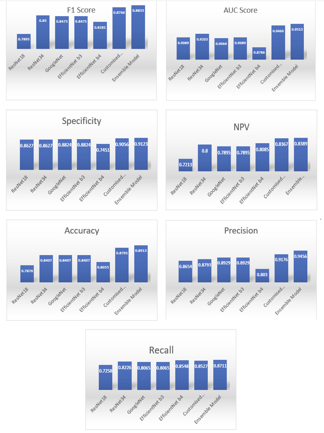
Figure 5. Performance evolution
5. CONCLUSION
Deep Convolutional Neural Networks (DCNNs) and Multiclass Support Vector Machines (MSVMs) offer promising approaches for classifying osteoporosis. DCNNs, renowned for their image classification prowess, can be trained on bone density scans or X-rays to learn intricate patterns and features indicative of healthy and osteoporotic bone. MSVMs, on the other hand, excel at finding optimal hyperplanes to separate different classes within a feature space. Training an MSVM on features extracted from bone images can effectively distinguish between healthy and osteoporotic conditions. The combined application of DCNNs and MSVMs holds significant potential. DCNNs can extract high-level features from images, which can then be fed into the MSVM for robust classification. This synergistic approach may enhance classification accuracy by leveraging the strengths of both techniques. However, several factors influence the success of this approach, including the quality of the training data, the careful selection of features, and the optimization of model parameters. Rigorous research and validation are crucial to establish the efficacy and reliability of this combined approach for accurate osteoporosis disease classification. Future work may require the integration of recurrent neural networks (RNNs) or transformer models with DCNNs and MSVMs for improved performance.
DATA AVAILABILITY STATEMENT
The data presented in this study are available on request from the corresponding author.
CONFLICTS OF INTEREST
The authors declare that they have no conflicts of interest in this work.
REFERENCES
[1] T. Sozen, L. Ozisik, and N. Calik Basaran, “An overview and management of osteoporosis,” Eur. J. Rheumatol., vol. 4, no. 1, pp. 46–56, Mar. 2017, doi: 10.5152/eurjrheum.2016.048.
[2] T. Suzuki and H. Yoshida, “Low bone mineral density at femoral neck is a predictor of increased mortality in elderly Japanese women,” Osteoporos. Int., vol. 21, no. 1, pp. 71–79, Jan. 2010, doi: 10.1007/s00198-009-0970-6.
[3] K. E. Ensrud et al., “Prevalent Vertebral Deformities Predict Mortality and Hospitalization in Older Women with Low Bone Mass,” J. Am. Geriatr. Soc., vol. 48, no. 3, pp. 241–249, Mar. 2000, doi: 10.1111/j.1532-5415.2000.tb02641.x.
[4] N. D. Nguyen, J. R. Center, J. A. Eisman, and T. V Nguyen, “Bone Loss, Weight Loss, and Weight Fluctuation Predict Mortality Risk in Elderly Men and Women,” J. Bone Miner. Res., vol. 22, no. 8, pp. 1147–1154, Aug. 2007, doi: 10.1359/jbmr.070412.
[5] P. J. Mitchell, “Fracture Liaison Services: the UK experience,” Osteoporos. Int., vol. 22, no. S3, pp. 487–494, Aug. 2011, doi: 10.1007/s00198-011-1702-2.
[6] S. J. Curry et al., “Screening for Osteoporosis to Prevent Fractures,” JAMA, vol. 319, no. 24, p. 2521, Jun. 2018, doi: 10.1001/jama.2018.7498.
[7] D. Mueller and A. Gandjour, “Cost-Effectiveness of Using Clinical Risk Factors with and without DXA for Osteoporosis Screening in Postmenopausal Women,” Value Heal., vol. 12, no. 8, pp. 1106–1117, Nov. 2009, doi: 10.1111/j.1524-4733.2009.00577.x.
[8] M. F. V. Sim, M. Stone, A. Johansen, and W. Evans, “Cost effectiveness analysis of BMD referral for DXA using ultrasound as a selective pre-screen in a group of women with low trauma Colles’ fractures,” Technol. Heal. Care, vol. 8, no. 5, pp. 277–284, Nov. 2000, doi: 10.3233/THC-2000-8503.
[9] C. A. Sedlak, M. O. Doheny, and S. L. Jones, “Osteoporosis Education Programs: Changing Knowledge and Behaviors,” Public Health Nurs., vol. 17, no. 5, pp. 398–402, Sep. 2000, doi: 10.1046/j.1525-1446.2000.00398.x.
[10] M. Sato, J. Vietri, J. A. Flynn, and S. Fujiwara, “Bone fractures and feeling at risk for osteoporosis among women in Japan: patient characteristics and outcomes in the National Health and Wellness Survey,” Arch. Osteoporos., vol. 9, no. 1, p. 199, Dec. 2014, doi: 10.1007/s11657-014-0199-7.
[11] A. Taguchi, “Triage screening for osteoporosis in dental clinics using panoramic radiographs,” Oral Dis., vol. 16, no. 4, pp. 316–327, May 2010, doi: 10.1111/j.1601-0825.2009.01615.x.
[12] D. A. Kumar and M. Anburajan, “The role of hip and chest radiographs in osteoporotic evaluation among south Indian women population: a comparative scenario with DXA,” J. Endocrinol. Invest., vol. 37, no. 5, pp. 429–440, May 2014, doi: 10.1007/s40618-014-0074-9.
[13] H. Chen, X. Zhou, H. Fujita, M. Onozuka, and K.-Y. Kubo, “Age-Related Changes in Trabecular and Cortical Bone Microstructure,” Int. J. Endocrinol., vol. 2013, pp. 1–9, 2013, doi: 10.1155/2013/213234.
[14] S. A. Holcombe, E. Hwang, B. A. Derstine, and S. C. Wang, “Measuring rib cortical bone thickness and cross section from CT,” Med. Image Anal., vol. 49, pp. 27–34, Oct. 2018, doi: 10.1016/j.media.2018.07.003.
[15] K. He, X. Zhang, S. Ren, and J. Sun, “Delving Deep into Rectifiers: Surpassing Human-Level Performance on ImageNet Classification,” in 2015 IEEE International Conference on Computer Vision (ICCV), IEEE, Dec. 2015, pp. 1026–1034. doi: 10.1109/ICCV.2015.123.
[16] J. Smets, E. Shevroja, T. Hügle, W. D. Leslie, and D. Hans, “Machine Learning Solutions for Osteoporosis—A Review,” J. Bone Miner. Res., vol. 36, no. 5, pp. 833–851, Dec. 2020, doi: 10.1002/jbmr.4292.
[17] T. P. Nguyen, D.-S. Chae, S.-J. Park, and J. Yoon, “A novel approach for evaluating bone mineral density of hips based on Sobel gradient-based map of radiographs utilizing convolutional neural network,” Comput. Biol. Med., vol. 132, p. 104298, May 2021, doi: 10.1016/j.compbiomed.2021.104298.
[18] C.-I. Hsieh et al., “Automated bone mineral density prediction and fracture risk assessment using plain radiographs via deep learning,” Nat. Commun., vol. 12, no. 1, p. 5472, Sep. 2021, doi: 10.1038/s41467-021-25779-x.
[19] N. Yamamoto et al., “Deep Learning for Osteoporosis Classification Using Hip Radiographs and Patient Clinical Covariates,” Biomolecules, vol. 10, no. 11, p. 1534, Nov. 2020, doi: 10.3390/biom10111534.
[20] B. Zhang et al., “Deep learning of lumbar spine X-ray for osteopenia and osteoporosis screening: A multicenter retrospective cohort study,” Bone, vol. 140, p. 115561, Nov. 2020, doi: 10.1016/j.bone.2020.115561.
[21] Ohta Y, Yamamoto K, Matsuzawa H, Kobayashi T, “Development of a fast screening method for osteoporosis using chest X-ray images and machine learning,” Can J Biomed Res Tech, vol. 3, no. 5, pp. 1–7, 2020.
[22] M. Jang, M. Kim, S. J. Bae, S. H. Lee, J.-M. Koh, and N. Kim, “Opportunistic Osteoporosis Screening Using Chest Radiographs With Deep Learning: Development and External Validation With a Cohort Dataset,” J. Bone Miner. Res., vol. 37, no. 2, pp. 369–377, Dec. 2020, doi: 10.1002/jbmr.4477.
[23] R. Yamashita, M. Nishio, R. K. G. Do, and K. Togashi, “Convolutional neural networks: an overview and application in radiology,” Insights Imaging, vol. 9, no. 4, pp. 611–629, Aug. 2018, doi: 10.1007/s13244-018-0639-9.
[24] N. Yamamoto et al., “Effect of Patient Clinical Variables in Osteoporosis Classification Using Hip X-rays in Deep Learning Analysis,” Medicina (B. Aires)., vol. 57, no. 8, p. 846, Aug. 2021, doi: 10.3390/medicina57080846.
[25] G. S. Collins, J. B. Reitsma, D. G. Altman, and K. G. M. Moons, “Transparent Reporting of a Multivariable Prediction Model for Individual Prognosis or Diagnosis (TRIPOD),” Circulation, vol. 131, no. 2, pp. 211–219, Jan. 2015, doi: 10.1161/CIRCULATIONAHA.114.014508.
[26] H. P. Dimai, “Use of dual-energy X-ray absorptiometry (DXA) for diagnosis and fracture risk assessment; WHO-criteria, T- and Z-score, and reference databases,” Bone, vol. 104, pp. 39–43, Nov. 2017, doi: 10.1016/j.bone.2016.12.016.
[27] K. He, X. Zhang, S. Ren, and J. Sun, “Deep Residual Learning for Image Recognition,” in 2016 IEEE Conference on Computer Vision and Pattern Recognition (CVPR), IEEE, Jun. 2016, pp. 770–778. doi: 10.1109/CVPR.2016.90.
[28] M. M. Mukaka, “Statistics corner: A guide to appropriate use of correlation coefficient in medical research.,” Malawi Med. J., vol. 24, no. 3, pp. 69–71, Sep. 2012.
[29] G. Liu, M. Peacock, O. Eilam, G. Dorulla, E. Braunstein, and C. C. Johnston, “Effect of osteoarthritis in the lumbar spine and hip on bone mineral density and diagnosis of osteoporosis in elderly men and women,” Osteoporos. Int., vol. 7, no. 6, pp. 564–569, Nov. 1997, doi: 10.1007/BF02652563.
[30] E. S. Siris et al., “Bone Mineral Density Thresholds for Pharmacological Intervention to Prevent Fractures,” Arch. Intern. Med., vol. 164, no. 10, p. 1108, May 2004, doi: 10.1001/archinte.164.10.1108.
[31] K. Vasu and S. Choudhary, “Music Information Retrieval Using Similarity Based Relevance Ranking Techniques,” Scalable Comput. Pract. Exp., vol. 23, no. 3, pp. 103–114, Oct. 2022, doi: 10.12694/scpe.v23i3.2005.
[32] V. Karthik and S. Choudhary, “TaCbF-‘Trending Architecture for Content based Filtering using Data Mining,’” in 2017 International Conference on Current Trends in Computer, Electrical, Electronics and Communication (CTCEEC), IEEE, Sep. 2017, pp. 417–420. doi: 10.1109/CTCEEC.2017.8455036.
BIOGRAPHIES OF AUTHORS

V. Santhi (Professor, VIT) has received her Ph.D. in Computer Science and Engineering from VIT University, Vellore, India. She has pursued her M.Tech. in Computer Science and Engineering from Pondicherry University, Puducherry. She has received her B.E. in Computer Science and Engineering from Bharathidasan University, Trichy, India. Currently, she is working as an Associate Professor in the School of Computing Science and Engineering at VIT University, Vellore, India. She has authored many national and international journal papers and one book. She is currently in the process of editing two books. Also, she has published many chapters in different books published by International publishers. She is a senior member of IEEE, and she is a member of many professional bodies like CSI, ISTE, IACSIT, IEEE, and IAENG. Her areas of research include Image Processing, Digital Signal Processing, Digital Watermarking, Data Compression, Data Mining and Computational Intelligence. She can be contacted at email: vsanthi@vit.ac.in.

T Ramesh is a research scholar at the School of Computer Science and Engineering, VIT University, Vellore, India. He has pursued his ME in Web Technology from the University Visvesvaraya College of Engineering, Bangalore University, Bangalore. He received his BTech in Computer Science and Information Technology from Jawaharlal Nehru Technological University, Hyderabad, India. Currently, he is working as an Assistant Professor in the Department of Computer Science and Engineering at Presidency University, Bangalore. He has published a few papers in international Journals and presented at a few National and International Conferences. His areas of research include Data Mining, Machine Learning. He can be contacted at email: t.ramesh2014@vit.ac.in.