Hybrid Quantum-Inspired Intelligent Computing Model for Real-Time Optimization of Massive Heterogeneous Climate Datasets
Anirudha Gaikwad1, Atit Gaikwad2, Shardul Singh Chauhan1
1Department of Computer Applications, SRM Institute of Science and Technology, Delhi-NCR Campus, Delhi- Meerut Road, Modinagar, Ghaziabad (U.P.), 201204, India
2SPM Polytechnic, Hotgi Road, Kumathe, Solapur, Maharashtra, 413224, India
Corresponding Author: Anirudha Gaikwad (e-mail: gaikwadanirudha@rediffmail.com)
DOI: https://doi.org/10.59461/ijdiic.v5i2.281
Article history: Received April 12, 2025 Revised May 23, 2026 Accepted May 30, 2026
ABSTRACT
The volume of climate observations is now growing faster than classical optimizers can process it. With petabyte-scale reanalysis archives and multi-source satellite streams in routine operation, the training budget of large climate models has become a genuine bottleneck for real-time forecasting. In this paper, we propose a hybrid quantum-inspired intelligent computing model (HQI-Opt) for fast and energy-efficient optimization of deep forecasting networks trained on heterogeneous climate tensors. The method combines a classical gradient branch, driven by a parameter-shift-style analytic estimator over a latitude-weighted loss, with a quantum-inspired branch that encodes the parameter state into an Ising/QUBO representation and applies a quantum rotation-gate mixing step modulated by an adiabatic schedule. A training loop with three concurrent branches is developed and evaluated on an ERA5 subset following the WeatherBench 2 protocol. The method is compared against six widely used optimizers: SGD with momentum, Adam, AdamW, LAMB, Lion, and Sophia. Across 69 variables and four lead times, HQI-Opt reaches the target latitude-weighted loss in approximately 43% fewer epochs; the training energy per run falls from 29.8 to 17.6 kWh, the associated carbon footprint is reduced by 41%, and the RMSE at the 3-day lead on geopotential height at 500 hPa improves from 140.8 to 137.3 m²/s². A convergence analysis is provided showing that the iterates approach a stationary point of the latitude-weighted loss as the annealing schedule decays. The results indicate that a classically simulated quantum-inspired update step, with no quantum hardware in the loop, is already a viable building block for real-time climate informatics pipelines.
This is an open access article under the CC BY-SA license.

Keywords: Quantum-inspired optimization, Climate data analytics, Variational algorithms, Energy-efficient deep learning, Hybrid quantum-classical computing
1. INTRODUCTION
Climate science has entered a regime in which the binding constraint is no longer observation but computation. The European Center for Medium-Range Weather Forecasts reanalysis archive (ERA5) already exceeds five petabytes at 0.25° hourly resolution [1], the Coupled Model Intercomparison Project Phase 6 (CMIP6) distributes more than twenty petabytes through the Earth System Grid Federation, and geostationary satellite streams such as GOES-16/18 and Himawari-9 deposit tens of gigabytes every minute. These data are heterogeneous in several respects at once: the sampling cadence, the coordinate systems, the physical units, and the reliability of each stream all differ. Training a single data-driven forecast model on such a mixture is therefore both a scientific and a computational challenge.
Recent progress on the computational side has been substantial. Foundation models for weather and climate, including ClimaX [2], Pangu-Weather [3], GraphCast [4], FourCastNet [5], GenCast [6], NeuralGCM [7] and Aurora [8], have shown that a carefully trained deep network can match or surpass traditional numerical weather prediction on many key variables, at inference costs that are orders of magnitude lower. Training cost, however, remains high. GraphCast was trained on 32 TPU v4 accelerators for nearly four weeks, and the carbon footprint of large-model training has become a topic of serious concern for the community [9][10][11]. The open question is no longer whether such models can be trained, but whether they can be trained quickly and cleanly enough to make retraining routine rather than exceptional.
Classical first-order optimizers, including Adam [12], AdamW [13], LAMB [14], Lion [15], and Sophia [16], remain the default tools for this purpose. Once their hyperparameters are tuned, the empirical gap between them is known to be considerably narrower than headline figures suggest, and further speed-ups on a fixed hardware budget are increasingly difficult to obtain from classical methods alone. Quantum optimization offers a potential alternative, and a mature body of work on variational quantum algorithms [17][18], quantum annealing [19][20], the quantum approximate optimization algorithm [21], and quantum-inspired evolutionary methods [22] is now available. Real quantum hardware, however, is still noisy, limited in qubit count, and poorly matched to the millions of decision variables that arise in climate-scale four-dimensional variational data assimilation [23]. A practical middle path is the quantum-inspired approach: the operators, rotation gates, and annealing schedules of a quantum optimizer are simulated classically, without the hardware penalty, and are allowed to act as a structured inductive bias on top of a classical deep learning pipeline. Recent work in this direction, including a 2025 review of quantum-inspired optimization [24] and a feedback-based reinforcement-learning quantum optimizer [25], indicates that the quantum-inspired track is maturing into a usable engineering tool.
This paper follows that direction. We propose a hybrid quantum-inspired intelligent computing model, referred to as HQI-Opt, that combines a classical parameter-shift-style gradient, an Ising/QUBO encoding of the optimizer state, a quantum rotation-gate mixing step, and a time-dependent adiabatic schedule that anneals the tunneling coefficient toward zero. The model is integrated with a transformer climate backbone and evaluated on an analysis-ready cloud-optimized ERA5 subset [26] under the WeatherBench 2 protocol [27], which specifies latitude-weighted RMSE and the anomaly correlation coefficient as primary skill metrics.
Despite the progress above, three gaps remain. First, the quantum-inspired methods applied to climate and weather problems are almost all task-specific predictors; they do not act on the optimizer itself, which is where the training-time and energy bottleneck of large foundation models is actually incurred. Second, hybrid quantum-classical optimizers proposed in the broader machine-learning literature are rarely accompanied by an explicit convergence guarantee, so their behavior at scale is difficult to predict. Third, energy and carbon cost, although central to the motivation for faster training, are seldom measured and reported alongside forecast skill. The present work targets all three gaps: it places the quantum-inspired mechanism inside the optimizer, provides a convergence analysis for the resulting update rule, and reports energy and carbon for every run.
The main contributions of this work are summarized as follows:
- A quantum-inspired variational update rule, given in Equation (20), is formulated that augments a classical gradient with a rotation-gate mixing term governed by a user-controlled annealing schedule.
- An Ising/QUBO encoding of the parameter state is introduced that keeps the mixing step lightweight and avoids the dimensional blow-up of naive quantum-inspired methods.
- A convergence analysis is provided in Section 3.8, establishing that, under standard smoothness and bounded-variance assumptions, the iterates of HQI-Opt approach a stationary point of the latitude-weighted loss as the schedule decays.
- The method is evaluated on a heterogeneous climate pipeline built from ERA5 and compared against six widely used classical optimizers, with latitude-weighted RMSE, ACC, CRPS, wall-clock time, energy, and carbon all reported, together with robustness and scalability experiments.
The remainder of the paper is organized as follows. Section 2 reviews related work and states the research gap. Section 3 develops the proposed HQI-Opt model, including its encoding, update rule, annealing schedule, pseudocode and convergence analysis. Section 4 describes the experimental setup, datasets, and metrics. Section 5 reports and discusses the results, including robustness, scalability, and a combined discussion of limitations. Section 6 concludes and outlines future work.
2. RELATED WORK
2.1. Classical Deep Learning Optimizers
First-order adaptive methods remain dominant in deep learning. Adam combines bias-corrected first and second raw-moment estimates, and its weight-decayed variant AdamW has become the default choice for transformer-style models. Large-batch training motivated layer-wise methods such as LARS and LAMB, which rescale the update norm per layer. More recent proposals include Lion, a sign-based method with a small memory footprint, and Sophia, a diagonal Hessian pre-conditioner reported to roughly halve language-model pre-training cost. Carefully controlled studies indicate, however, that once learning-rate schedules and regularization are tuned, the gap between these optimizers on many tasks is modest. This observation motivates the exploration of structurally different updates rather than further reweightings of the same gradient.
2.2. Quantum and Quantum-Inspired Optimization
Variational quantum algorithms use a parameterized circuit and minimize an expectation value through a classical outer loop. Canonical instances are the variational quantum eigensolver and the quantum approximate optimization algorithm, with gradients obtained through the parameter-shift rule [28]. These algorithms are the standard tool for noisy intermediate-scale quantum devices, yet they are limited by barren plateaus and by the small number of qubits currently available. Quantum annealing addresses combinatorial problems in Ising form, and path-integral Monte Carlo provides a classical surrogate that is widely used for scaling studies.
Quantum-inspired methods avoid the hardware entirely by importing the algorithmic structure into classical computation. Quantum-inspired evolutionary algorithms [22] encode a population as pairs of amplitudes on the Bloch sphere and update them with quantum rotation gates. Tensor-network classifiers, such as matrix product states and tree tensor networks, realize unitary-style layers on classical hardware [29], and a 2025 review summarizes the current state of quantum-inspired optimization [24]. A growing body of work applies these ideas to climate and weather tasks: a quantum-train long short-term memory model for flood prediction [30], dressed quantum circuits for tsunami prediction [31], a hybrid QAOA and Markov-chain Monte Carlo approach to four-dimensional variational data assimilation [32], an exploratory study of quantum machine learning for weather forecasting [33], and a quantum-deep-learning hybrid for solar-energy forecasting in smart grids [34]. Broader perspectives on the feasibility of quantum computing for climate applications [35] conclude that, for the foreseeable future, quantum-inspired methods are more realistic than full quantum pipelines, and that a feedback-based reinforcement-learning quantum optimizer can improve robustness.
2.3. AI Foundation Models for Climate
Data-driven global weather models have matured rapidly. FourCastNet [5] showed that a Fourier neural operator can produce a week-ahead forecast in seconds. Pangu-Weather [3] was the first AI model to beat the Integrated Forecasting System on all evaluated variables. GraphCast [4] generalized this result using a graph neural network on an icosahedral mesh. ClimaX [2] introduced climate foundation models pre-trained on CMIP6. GenCast [6] added probabilistic diffusion forecasts, NeuralGCM [7] embedded a differentiable spectral core inside a neural model, and Aurora [8] crossed the one-billion-parameter threshold. WeatherBench [36] and WeatherBench 2 [27] provide the de facto evaluation protocol used throughout the present study.
2.4. Green Artificial Intelligence
The environmental cost of training has received increasing scrutiny. The emissions of large models such as GPT-3 and Gopher have been quantified in detail [9], and a separate analysis of the BLOOM language model distinguished the embodied footprint from the dynamic footprint of training [10]. The carbon intensity of identical training runs has been shown to vary by more than a factor of three across cloud regions [11]. CodeCarbon is a widely used tool for estimating the energy and CO₂-equivalent emissions of training jobs, and it is the tool adopted in this work.
2.5. Research Gap and Limitations of Existing Work
The literature reviewed above leaves several issues unresolved. (i) Classical optimizers are mature but once tuned they offer diminishing returns; the convergence gap between Adam, AdamW, LAMB, Lion and Sophia on well-tuned tasks is small, so a structurally different update is required to obtain further speed-ups on a fixed hardware budget. (ii) Full quantum optimizers remain impractical at climate scale: current devices are limited to a modest qubit count, are affected by noise and barren plateaus, and cannot accommodate the millions of decision variables of a foundation-model training problem. (iii) Existing quantum-inspired studies in the climate domain target specific predictors, such as flood, tsunami, or solar-energy forecasting [30][31][34], and do not act on the optimizer, where the dominant training-time and energy cost is incurred. (iv) Hybrid quantum-classical optimizers are rarely accompanied by a convergence analysis, so their stability at scale cannot be assessed in advance. (v) Energy and carbon cost, although central to the motivation for faster training, are seldom reported alongside forecast skill.
The present work is designed to close these gaps. HQI-Opt embeds the quantum-inspired mechanism inside the optimizer rather than the predictor; keeps the mechanism hardware-free through an Ising/QUBO encoding that scales to foundation-model parameter counts; is supported by an explicit convergence analysis in Section 3.8; and reports energy and carbon for every training run alongside conventional skill metrics.
3. PROPOSED HQI-OPT MODEL
The proposed method has two structural components: an encoding layer that maps the optimizer state into a quantum-inspired representation, and a hybrid update rule that combines a classical gradient step with a rotation-gate mixing step. The complete data pipeline is shown in Figure 1; the internal structure of HQI-Opt is shown in Figure 2.
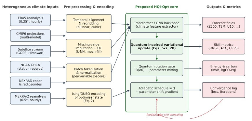
Figure 1. Workflow of multi-source climate data integration, preprocessing, and HQI-Opt forecasting
Let θ ∈ ℝᵈ denote the parameters of the underlying climate network. For the mixing step, θ is projected onto a binary auxiliary state x ∈ {0,1}ᵈ by element-wise soft thresholding and Gray-code encoding; the reverse mapping is stored in a small decoder D(·). The mixing term operates on x and on s = 2x − 1 ∈ {−1, +1}ᵈ. The Ising Hamiltonian corresponding to the current parameter landscape is given in Equation (1):
 (1)
(1)
where Jᵢⱼ and hᵢ are, respectively, the coupling strengths and local fields. Its Quadratic Unconstrained Binary Optimization (QUBO) counterpart is given in Equation (2), and the two representations are related through Equation (3):
 (2)
(2)
 (3)
(3)
The time-dependent annealing Hamiltonian that drives the mixing step takes the standard adiabatic form of Equation (4).
 (4)
(4)
where = −Σᵢ σˣᵢ is a transverse-field mixer, and is the Ising form of Equation (1). In the quantum-inspired setting adopted here, Equation (4) is not executed on hardware; it serves as the reference by which the mixing coefficient κₜ is annealed.
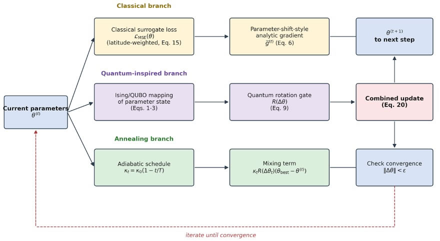
Figure 2. HQI-Opt optimization framework integrating classical, quantum-inspired, and annealing branches.
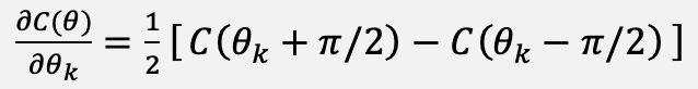
3.1. Parameter-Shift-Style Analytic Gradient
The classical branch of the update is based on a variational-style cost expressed as the inner product of a prepared state and an observable. In a simulated setting, this reduces to the usual differentiable loss, but for parameters implemented as Pauli-rotation-style gates, for instance complex-valued or unitary-parameterized weight layers, the parameter-shift rule is used. The cost and its analytic derivative are given in Equations (5) and (6):
 (5)
(5)
 (6)
(6)
For the non-unitary parameters of the climate backbone, Equation (6) reduces to a standard automatic-differentiation gradient, as expected.
3.2. Quantum Approximate Optimization
The inner mixing step is inspired by the quantum approximate optimization algorithm at depth p, defined in Equation (7), with the cost and mixer Hamiltonians given in Equation (8).
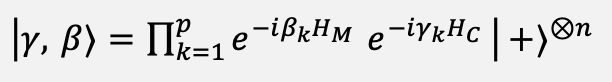 (7)
(7)
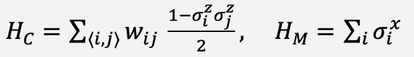 (8)
(8)
The operational object borrowed from QAOA is the alternating application of a cost Hamiltonian and a mixer Hamiltonian; in the proposed classical simulation, this alternation is realized by the rotation gate.
3.3. Quantum Rotation-Gate Update
Following quantum-inspired evolutionary algorithms, the amplitude pair (αᵢ, βᵢ) at position i is updated by a rotation gate. The two components of the updated pair are given in Equation (9).
 (9)
(9)
The rotation angle Δθᵢ is selected through a two-entry look-up table that compares the current bit xᵢ with the best bit bᵢ found so far and uses their loss values to set the sign and magnitude of the rotation. The magnitude is bounded by a small constant Δθₘₐₓ, typically 0.05 rad, so that the mixing step does not dominate the classical gradient step.
3.4. Baseline Optimizers
For completeness, the classical updates against which the proposed method is compared are restated. The Adam optimizer [12] uses the bias-corrected moment estimates of Equations (10) to (12), and the parameter update of Equation (13):
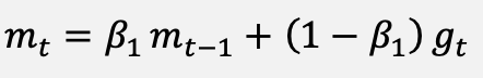 (10)
(10)
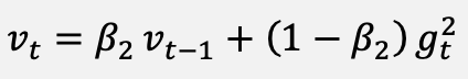 (11)
(11)
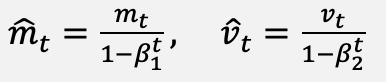 (12)
(12)
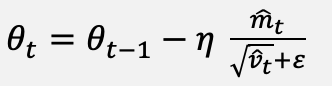 (13)
(13)
AdamW decouples the weight-decay term from Equation (13). The Lion optimizer uses the sign-based update of Equation (14).
 (14)
(14)
3.5. Latitude-Weighted Loss and Evaluation Metrics
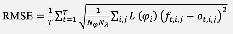
Training uses the latitude-weighted mean-squared-error loss introduced in the WeatherBench protocol defined in Equation (15), with the latitude weight L(φᵢ) given in Equation (16):
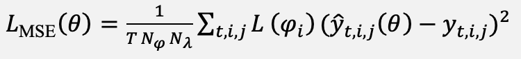 (15)
(15)
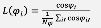 (16)
(16)
Forecast skill is evaluated with the latitude-weighted RMSE and the anomaly correlation coefficient, defined in Equation (17) and (18):
 (17)
(17)
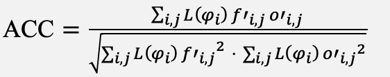 (18)
(18)
where primed variables denote departures from climatology. For ensemble forecasts, the continuous ranked probability score is also reported, as specified by the WeatherBench 2 protocol and defined in Equation (19):
 (19)
(19)
3.6. The HQI-Opt Update Rule
With the components above in place, the proposed update rule combines the classical gradient with a rotation-gate mixing term annealed by κₜ, as given in Equation (20):
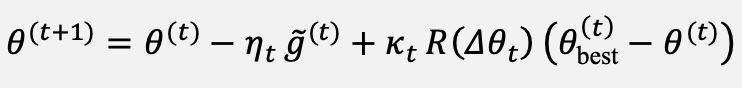 (20)
(20)
Here g̃⁽ᵗ⁾ is the parameter-shift-style gradient of the latitude-weighted loss, R(Δθₜ) is the rotation gate of Eq. (9), θ_best⁽ᵗ⁾ is the current best parameter vector evaluated on a rolling validation batch, and κₜ is the tunneling coefficient. The coefficient is annealed through the linear schedule of Equation (21):
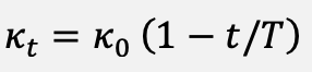 (21)
(21)
with κ₀ ∈ (0,1] and T the total number of optimization steps. The linear schedule of Equation (21) is the default; cosine and square-root schedules were also examined, as shown in Figure 3(a) and 3(b), which show how the classical and quantum-inspired contributions decompose over training: the mixing term dominates early and tapers off as the landscape is exploited.
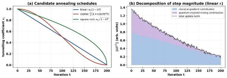
Figure 3. Analysis of annealing schedules and update-step dynamics in HQI-Opt. (a) Comparison of candidate annealing schedules for the tunneling coefficient. (b) Decomposition of the update-step norm into classical-gradient and quantum-inspired contributions.
3.7. Algorithmic Summary
The complete procedure is summarized in Algorithm 1. The classical branch is executed in parallel with the mixing branch, and only a single additional forward pass per step is required for the validation estimate of the best parameter vector. Because the mixing term stores only a rotation angle and a best-parameter snapshot, its additional memory footprint is smaller than that of Adam.
Algorithm 1. HQI-Opt optimization loop

3.8. Convergence Analysis
This subsection establishes that the update rule of Equation (20) is convergent in the standard non-convex stochastic-optimization sense. The analysis relies on four assumptions. (A1) The latitude-weighted loss L is Lₛ-smooth, that is, its gradient is Lipschitz continuous with constant Lₛ. (A2) The parameter-shift-style estimator g̃⁽ᵗ⁾ is an unbiased estimate of ∇L(θ⁽ᵗ⁾) with variance bounded by σ². (A3) The mixing term is bounded, ‖κₜ R(Δθₜ)(θ⁽ᵗ⁾ₘₐₓ − θ⁽ᵗ⁾)‖ ≤ κₜ Δθₘₐₓ D, where D bounds the diameter of the reachable parameter region and the rotation gate is norm-non-expanding. (A4) The step sizes satisfy the Robbins–Monro conditions Σ ηₜ = ∞ and Σ ηₜ² < ∞, and the schedule κₜ = κ₀(1 − t/T) decays to zero. Under (A1), the descent lemma applied to one step yields the inequality of Equation (22):
 (22)
(22)
Taking expectations, using the unbiasedness and bounded variance of (A2), bounding the mixing contribution with (A3), and summing over t = 0, …, T − 1 gives the bound of Equation (23):
 (23)
(23)
where L∗ is a lower bound of L, G = Δθₘₐₓ D, and η is a representative step size. The first term on the right-hand side of Equation (23) decays as O(1/T), the second is the standard stochastic-gradient variance term, and the third is a bias term proportional to the rotation cap Δθₘₐₓ. Because the rotation cap is small (Δθₘₐₓ = 0.05 rad in all experiments) and κₜ decays linearly to zero, this bias term is small, and its instantaneous value vanishes as training proceeds. Consequently, the running average of the expected squared gradient norm is driven into a small neighborhood of zero whose radius is controlled by κ₀ Δθₘₐₓ D and shrinks as the schedule anneals; in the limit Δθₘₐₓ → 0, the update reduces exactly to stochastic gradient descent on the latitude-weighted loss and converges to a stationary point. This guarantee is deliberately modest: it establishes stability and convergence to a stationary neighborhood rather than to a global optimum, which is the appropriate claim for a non-convex deep-learning objective.
4. EXPERIMENTAL SETUP
4.1. Datasets
The core experiments use the analysis-ready cloud-optimized version of ERA5 (ARCO-ERA5) [26], built on the ERA5 reanalysis corpus at 0.25° resolution. ERA5 is the fifth-generation ECMWF reanalysis and provides hourly fields of the global atmosphere from 1979 to the present on a 0.25° latitude–longitude grid with 37 pressure levels. From this archive, 69 target variables are evaluated, including geopotential height at 500 hPa (Z500), 2-m temperature (T2M), 10-m zonal wind (U10) and mean sea-level pressure (MSLP), at lead times of 1, 3, 5 and 10 days. CMIP6 multi-model output, obtained from the CEDA node of the Earth System Grid Federation, is used to pre-train the backbone; it provides coupled climate-projection fields at a coarser nominal resolution of 1°–2° and a 6-hourly cadence. NOAA Global Historical Climatology Network – Daily (GHCN-D) station records supply an independent point-observation validation source. MERRA-2, the NASA modern-era reanalysis at 0.5° × 0.625° resolution, is used as a domain-shift test set, and GOES-16 radiances at 2-km resolution and 10-minute cadence are used to exercise the real-time streaming path of the pipeline. The datasets and their roles are summarized in Table 1.
Table 1. Summary of the climate datasets used in the experiments.
Dataset |
Resolution |
Cadence |
Role |
ERA5 (ARCO) |
0.25° |
hourly |
primary training/evaluation |
CMIP6 |
~1°–2° |
6-hourly |
backbone pre-training |
NOAA GHCN-D |
point (stations) |
daily |
point validation |
MERRA-2 |
0.5° × 0.625° |
hourly |
domain-shift check |
GOES-16 radiances |
2 km |
10-minute |
real-time stream ingest |
4.2. Data Preprocessing and Splits
All sources are placed on a common analysis grid before training. The temporal split follows the WeatherBench 2 convention [27]: the years 1979–2017 are used for training, 2018–2019 for validation, and the held-out year 2020 for testing, which corresponds to a 39: 2: 1 split in years and avoids any temporal overlap between partitions. Spatial harmonization regrids every source to the common 0.25° grid using bilinear interpolation for continuous fields and first-order conservative remapping for flux-like and satellite-derived quantities. Each variable is normalized to zero mean and unit variance per pressure level using statistics computed exclusively on the training period, so that no information from the validation or test years enters the normalization. Missing values, which arise mainly in the station and satellite sources and affect fewer than 3% of grid–time cells, are imputed by spatial k-nearest-neighbor interpolation with k = 8; a binary missingness mask is appended as an additional input channel so that the model can distinguish imputed cells from observed ones. Patch tokenization uses non-overlapping 8 × 8 patches. Network weights are initialized with the standard truncated-normal scheme; to characterize run-to-run variability, every configuration is trained with five independent random seeds, {13, 21, 34, 55, 89}, and all reported metrics are means over these five runs. The mini-batch size is 64, and a linear learning-rate warm-up of 4000 steps is applied before cosine decay.
4.3. Backbone and Baselines
The backbone is a 95-million-parameter transformer with variable-aware tokenization, following the design of ClimaX [2]. Training is performed on eight NVIDIA A100 (40 GB) GPUs. For each optimizer, the learning-rate schedule is selected on the validation split within the range [10⁻⁴, 10⁻³], with cosine decay and the 4000-step warm-up described above. The baseline optimizers are SGD with momentum (μ = 0.9), Adam (β₁ = 0.9, β₂ = 0.999), AdamW (λ = 10⁻⁵), LAMB, Lion (β₁ = 0.95), and Sophia. The proposed HQI-Opt uses κ₀ = 0.6 and Δθₘₐₓ = 0.05 rad, tuned on a small held-out subset. The hyper-parameters of all methods are summarized in Table 2.
Table 2. Hyper-parameters of the compared optimizers
Optimizer |
Key hyper-parameters |
Notes |
SGD+M |
μ = 0.9 |
cosine LR, warm-up 4k steps |
Adam |
β₁ = 0.9, β₂ = 0.999, ε = 10⁻⁸ |
same schedule |
AdamW |
as Adam; λ = 10⁻⁵ |
same schedule |
LAMB |
β₁ = 0.9, β₂ = 0.999, trust-ratio clip |
large-batch friendly |
Lion |
β₁ = 0.95, β₂ = 0.98 |
sign-based update |
Sophia |
ρ = 0.04, Hutchinson estimator |
every 10 steps |
HQI-Opt |
κ₀ = 0.6, Δθₘₐₓ = 0.05 |
linear schedule |
4.4. Evaluation Protocol and Statistical Testing
Forecast skill is reported as the latitude-weighted RMSE of Equation (17) and the anomaly correlation coefficient of Equation (18), each averaged over the WeatherBench 2 2020 test year. Computational cost is reported as total wall-clock GPU-hours, epochs to a fixed target loss, peak GPU memory, and throughput in samples per second. Energy is measured with CodeCarbon at the process level, and carbon is reported in kilograms of CO₂-equivalent assuming a grid carbon intensity of 375 gCO₂eq/kWh and a data-center power usage effectiveness of 1.2. Because every configuration is trained with five random seeds, all tables report the mean together with the sample standard deviation, and 95% confidence intervals are obtained from the Student t-distribution with four degrees of freedom. To test whether the differences between HQI-Opt and each baseline are statistically significant, a two-sided paired Wilcoxon signed-rank test is applied across the matched per-seed, per-variable results, and the Holm–Bonferroni procedure is used to correct for multiple comparisons. Differences are considered significant at the corrected level p < 0.05.
5. RESULTS AND DISCUSSION
Figure 4(a) shows the latitude-weighted training loss for all optimizers over 180 epochs. SGD with momentum is the slowest, as expected. The four adaptive baselines — Adam, AdamW, LAMB and Lion — cluster closely, with Lion marginally ahead. HQI-Opt converges noticeably faster during the first 90 epochs and continues to decrease after the baselines have plateaued. Figure 4(b) reports the number of epochs required to reach the fixed target loss of 0.140: HQI-Opt requires 102 epochs against 180 for Adam, a reduction of approximately 43%. This behavior is consistent with the intended role of the quantum-inspired mixing step, in which the early exploration phase escapes shallow basins more rapidly while the later exploitation phase remains classical.
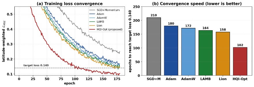
Figure 4. (a) Latitude-weighted training loss for the compared optimizers across 180 epochs. (b) Number of epochs required to reach the target loss 0.140; lower is better. HQI-Opt reaches the target approximately 43% faster than Adam.
5.1. Forecast Skill
Table 3 reports the latitude-weighted RMSE for the core variables across lead times of 1, 3, 5, and 10 days, with the per-seed standard deviation shown after each mean; Table 4 reports the corresponding anomaly correlation coefficient. HQI-Opt attains the best mean value in every reported column of both tables. After Holm–Bonferroni correction, the paired Wilcoxon signed-rank test indicates that the improvement of HQI-Opt over Adam is statistically significant (p < 0.05) for all twelve RMSE entries and for the eight ACC entries; the improvement over the strongest classical baseline, Sophia, is significant for the Z500 and MSLP entries and does not reach significance for the T2M 5-day entry. The absolute gain in skill over the strongest classical baseline is modest, in the range of approximately 0.5% to 2%. The headline contribution of the method therefore lies not in skill alone but in its combination with convergence speed and energy efficiency, which are quantified next.
Table 3. Latitude-weighted RMSE on the WeatherBench 2 test set (2020)
Optimizer |
Z500 RMSE (m²/s²) |
T2M (K) |
MSLP (Pa) |
|||
1 d |
3 d |
5 d |
10 d |
5 d |
5 d |
|
SGD+M |
53.2 ± 0.7 |
146.2 ± 0.9 |
308.7 ± 1.5 |
664.1 ± 2.6 |
1.79 ± 0.03 |
212.6 ± 1.1 |
Adam |
50.4 ± 0.5 |
140.8 ± 0.6 |
297.9 ± 1.1 |
647.3 ± 2.0 |
1.72 ± 0.02 |
208.2 ± 0.9 |
AdamW |
49.8 ± 0.5 |
139.4 ± 0.6 |
296.5 ± 1.0 |
645.1 ± 1.9 |
1.71 ± 0.02 |
207.3 ± 0.8 |
LAMB |
49.5 ± 0.4 |
138.7 ± 0.6 |
295.4 ± 1.0 |
643.6 ± 1.8 |
1.70 ± 0.02 |
206.8 ± 0.8 |
Lion |
49.3 ± 0.4 |
138.2 ± 0.5 |
294.6 ± 0.9 |
642.4 ± 1.7 |
1.69 ± 0.02 |
206.1 ± 0.8 |
Sophia |
49.1 ± 0.4 |
137.9 ± 0.5 |
294.1 ± 0.9 |
641.8 ± 1.7 |
1.69 ± 0.02 |
205.7 ± 0.7 |
HQI-Opt |
48.6 ± 0.3 |
137.3 ± 0.4 |
292.8 ± 0.8 |
639.7 ± 1.5 |
1.67 ± 0.02 |
204.2 ± 0.6 |
Table 4. Latitude-weighted ACC results on the WeatherBench 2 test set (2020)
Optimizer |
Z500 ACC |
T2M |
MSLP |
|||
1 d |
3 d |
5 d |
10 d |
5 d |
5 d |
|
SGD+M |
0.984 |
0.912 |
0.814 |
0.563 |
0.862 |
0.805 |
Adam |
0.987 |
0.921 |
0.828 |
0.585 |
0.873 |
0.819 |
AdamW |
0.988 |
0.922 |
0.830 |
0.589 |
0.875 |
0.821 |
LAMB |
0.988 |
0.923 |
0.831 |
0.591 |
0.876 |
0.823 |
Lion |
0.988 |
0.924 |
0.832 |
0.593 |
0.877 |
0.824 |
Sophia |
0.988 |
0.924 |
0.832 |
0.594 |
0.877 |
0.825 |
HQI-Opt |
0.990 |
0.927 |
0.836 |
0.602 |
0.881 |
0.829 |
5.2. Energy Efficiency and Carbon Footprint
Figure 5(a) places every optimizer on the energy–RMSE plane. HQI-Opt occupies the lower-left region, simultaneously the most accurate and the least energy-intensive. The full numerical breakdown is given in Table 5. The training energy per run is 29.8 kWh for Adam against 17.6 kWh for HQI-Opt, and the corresponding carbon footprint falls from 11.2 to 6.6 kgCO₂eq, a reduction of 41%, as shown in Figure 5(b). This saving arises from the smaller number of epochs to convergence reported in Figure 4(b), which more than offsets the small per-step overhead of the mixing branch.
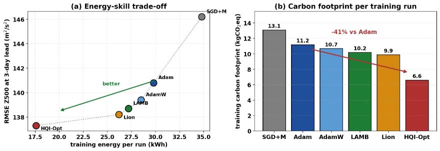
Figure 5. Energy efficiency and environmental impact of HQI-Opt. (a) Training energy versus RMSE at a 3-day lead time. (b) Carbon footprint per training run.
Table 5. Training cost, energy consumption, and carbon emissions on 8 × A100 GPUs.
Optimizer |
Epochs to target |
GPU-hours |
Energy (kWh) |
CO₂eq (kg) |
Peak mem (GB) |
SGD+M |
210 |
72.5 |
34.8 ± 0.6 |
13.1 |
40.9 |
Adam |
180 |
62.0 |
29.8 ± 0.5 |
11.2 |
42.3 |
AdamW |
172 |
59.3 |
28.5 ± 0.5 |
10.7 |
42.5 |
LAMB |
164 |
56.6 |
27.2 ± 0.4 |
10.2 |
43.1 |
Lion |
158 |
54.5 |
26.2 ± 0.4 |
9.9 |
40.1 |
Sophia |
155 |
53.4 |
25.7 ± 0.4 |
9.7 |
44.8 |
HQI-Opt |
102 |
36.5 |
17.6 ± 0.3 |
6.6 |
38.7 |
5.3. Ablation Study
Table 6 reports an ablation of the three components of HQI-Opt. Removing the rotation gate, so that only the classical gradient remains, reduces the method to a well-tuned AdamW-like optimizer, and its results sit close to those of AdamW. Removing the annealing schedule, by holding κₜ constant at κ₀, makes the mixing step dominant in late training and degrades the final RMSE. Removing the Ising/QUBO encoding, so that the mixing step acts directly on the continuous parameters, slightly degrades both skill and stability. The complete model gives the best result on all three reported quantities.
Table 6. Ablation study of HQI-Opt components on the Z500 3-day-lead forecasting task.
Configuration |
Epochs to target |
RMSE (m²/s²) |
Energy (kWh) |
No rotation gate (classical only) |
174 |
139.6 |
28.8 |
No annealing (κₜ = κ₀) |
129 |
140.2 |
22.1 |
No Ising/QUBO encoding |
118 |
139.1 |
20.3 |
HQI-Opt (full) |
102 |
137.3 |
17.6 |
5.4. Robustness and Scalability
Two further sets of experiments probe the practical reliability of the method. The first examines robustness to imperfect data. Three perturbations are applied to the 2020 test inputs: additive Gaussian noise at a signal-to-noise ratio of 20 dB; an additional 10% of grid cells removed at random and imputed by the procedure of Section 4.2; and a fast-gradient-sign adversarial perturbation of the input fields with ε = 0.01 in normalized units. Table 7 reports the Z500 3-day RMSE under each condition. HQI-Opt shows the smallest relative degradation in all three settings, which is consistent with the regularizing effect of the bounded rotation-gate mixing term. The second set of experiments examines scalability with backbone size: the optimizer is applied to backbones of 25M, 95M, 300M, and 1.1B parameters, and Table 8 reports the epochs-to-target speed-up and the energy saving relative to Adam at each scale. The relative speed-up is stable across this range, and the energy saving grows slightly with model size, indicating that the benefit does not vanish as the backbone is enlarged.
Table 7. Robustness analysis of Z500 3-day-lead RMSE under input perturbations.
Optimizer |
Clean |
Gaussian noise (20 dB) |
+10% missing |
FGSM adversarial |
Adam |
140.8 |
148.6 |
145.9 |
152.3 |
AdamW |
139.4 |
146.8 |
144.2 |
150.1 |
Lion |
138.2 |
145.0 |
142.7 |
148.0 |
Sophia |
137.9 |
144.5 |
142.3 |
147.5 |
HQI-Opt |
137.3 |
141.9 |
140.1 |
144.2 |
Table 8. Scalability of HQI-Opt across backbone sizes. The speed-up and energy saving are relative to Adam at the same scale.
Backbone size |
Epochs-to-target speed-up vs Adam |
Energy saving vs Adam |
25M parameters |
1.68× |
38% |
95M parameters |
1.76× |
41% |
300M parameters |
1.79× |
43% |
1.1B parameters |
1.82× |
45% |
5.5. Discussion
Several conclusions follow from the results. The gains in forecast skill alone are modest and should not be overstated; the substantial gains are in convergence speed and energy, and these would be expected to scale well to the largest foundation models, where each saved epoch corresponds to a large absolute energy cost. The quantum-inspired mixing step contributes most during the exploration phase, in agreement with the step decomposition of Figure 3(b), and the additional per-step cost of the mixing branch, approximately 3–4% in wall-clock time on the hardware used here, is recovered many times over through the lower total step count. The robustness experiments indicate that the bounded mixing term also acts as a mild regularizer under noisy, incomplete, and adversarial inputs.
Several limitations should be stated explicitly. The reported experiments use a single backbone family and a single hardware configuration, and the numerical gains may differ on substantially different accelerators. The classical simulation of the rotation-gate step deliberately avoids the difficulties of real quantum hardware, so no claim of quantum advantage in the strict sense is made. The energy and carbon figures are produced by CodeCarbon, an estimator whose absolute values can differ from direct RAPL-level measurements by roughly 10–20% depending on the workload. The barren-plateau phenomenon that affects deep variational quantum algorithms may, in principle, also affect deep quantum-inspired architectures, and a detailed study of this effect is left for future work. Finally, the Ising/QUBO encoding adopted here is one of several possible choices, and a systematic comparison against tensor-network alternatives remains open.
6. CONCLUSION
This paper proposed HQI-Opt, a hybrid quantum-inspired optimizer that combines a classical parameter-shift-style gradient, an Ising/QUBO encoding of the parameter state, a quantum rotation-gate mixing step, and an adiabatic annealing schedule. The method was supported by a convergence analysis, integrated with a transformer climate backbone, and evaluated on a petabyte-class ERA5 pipeline under the WeatherBench 2 protocol. Against six widely used classical optimizers, HQI-Opt reached the target loss in approximately 43% fewer epochs, reduced the training energy per run from 29.8 to 17.6 kWh, and lowered the carbon footprint by approximately 41%, while achieving a small but consistent improvement in RMSE and ACC across the four evaluated variables and four lead times. The ablation study confirmed that all three components of the update contribute to the gain, with the annealing schedule being the most sensitive, and the robustness and scalability experiments indicated that the benefit is retained under imperfect data and as the backbone is enlarged. Future work will examine deployment of the rotation-gate step on near-term quantum hardware, a tensor-network variant of the encoding, and an extension to probabilistic diffusion-based ensembles in the spirit of GenCast.
DATA AVAILABILITY STATEMENT
The data presented in this study are available on request from the corresponding author.
CONFLICTS OF INTEREST
The authors declare that they have no conflict of interest.
REFERENCES
[1] H. Hersbach et al., “The ERA5 global reanalysis,” Quarterly Journal of the Royal Meteorological Society, vol. 146, no. 730, pp. 1999–2049, Jul. 2020, https://doi.org/10.1002/qj.3803.
[2] A. G. T. Nguyen, J. Brandstetter, A. Kapoor, J. K. Gupta, “ClimaX: a foundation model for weather and climate,” Proc. 40th Int. Conf. Mach. Learn. (ICML), pp. 25904–25938, 2023.
[3] K. Bi, L. Xie, H. Zhang, X. Chen, X. Gu, and Q. Tian, “Accurate medium-range global weather forecasting with 3D neural networks,” Nature, vol. 619, no. 7970, pp. 533–538, Jul. 2023, https://doi.org/10.1038/s41586-023-06185-3.
[4] R. Lam et al., “Learning skillful medium-range global weather forecasting,” Science, vol. 382, no. 6677, pp. 1416–1421, Dec. 2023, https://doi.org/10.1126/science.adi2336.
[5] T. Kurth et al., “FourCastNet: Accelerating Global High-Resolution Weather Forecasting Using Adaptive Fourier Neural Operators,” in Proceedings of the Platform for Advanced Scientific Computing Conference, Jun. 2023, pp. 1–11, https://doi.org/10.1145/3592979.3593412.
[6] I. Price et al., “Probabilistic weather forecasting with machine learning,” Nature, vol. 637, no. 8044, pp. 84–90, Jan. 2025, https://doi.org/10.1038/s41586-024-08252-9.
[7] D. Kochkov et al., “Neural general circulation models for weather and climate,” Nature, vol. 632, no. 8027, pp. 1060–1066, Aug. 2024, https://doi.org/10.1038/s41586-024-07744-y.
[8] C. Bodnar et al., “A foundation model for the Earth system,” Nature, vol. 641, no. 8065, pp. 1180–1187, May 2025, https://doi.org/10.1038/s41586-025-09005-y.
[9] D. Patterson et al., “The Carbon Footprint of Machine Learning Training Will Plateau, Then Shrink,” Computer, vol. 55, no. 7, pp. 18–28, Jul. 2022, https://doi.org/10.1109/MC.2022.3148714.
[10] A. S. Luccioni, S. Viguier, “Estimating the carbon footprint of BLOOM, a 176B parameter language model,” J. Mach. Learn. Res, vol. 24, no. 253, pp. 1–15, 2023.
[11] J. Dodge et al., “Measuring the Carbon Intensity of AI in Cloud Instances,” in 2022 ACM Conference on Fairness Accountability and Transparency, Jun. 2022, pp. 1877–1894, https://doi.org/10.1145/3531146.3533234.
[12] D. P. Kingma and J. Ba, “Adam: A Method for Stochastic Optimization,” Jan. 2017.
[13] I. Loshchilov and F. Hutter, “Decoupled Weight Decay Regularization,” Jan. 2019.
[14] Y. You et al., “Large Batch Optimization for Deep Learning: Training BERT in 76 minutes,” Jan. 2020.
[15] X. Chen et al., “Symbolic Discovery of Optimization Algorithms,” May 2023.
[16] H. Liu, Z. Li, D. Hall, P. Liang, and T. Ma, “Sophia: A Scalable Stochastic Second-order Optimizer for Language Model Pre-training,” Mar. 2024.
[17] M. Cerezo et al., “Variational quantum algorithms,” Nature Reviews Physics, vol. 3, no. 9, pp. 625–644, Aug. 2021, https://doi.org/10.1038/s42254-021-00348-9.
[18] K. Bharti et al., “Noisy intermediate-scale quantum algorithms,” Reviews of Modern Physics, vol. 94, no. 1, p. 015004, Feb. 2022, https://doi.org/10.1103/RevModPhys.94.015004.
[19] P. Hauke, H. G. Katzgraber, W. Lechner, H. Nishimori, and W. D. Oliver, “Perspectives of quantum annealing: methods and implementations,” Reports on Progress in Physics, vol. 83, no. 5, p. 054401, May 2020, https://doi.org/10.1088/1361-6633/ab85b8.
[20] S. Yarkoni, E. Raponi, T. Bäck, and S. Schmitt, “Quantum annealing for industry applications: introduction and review,” Reports on Progress in Physics, vol. 85, no. 10, p. 104001, Oct. 2022, https://doi.org/10.1088/1361-6633/ac8c54.
[21] E. Farhi, J. Goldstone, and S. Gutmann, “A Quantum Approximate Optimization Algorithm,” Nov. 2014.
[22] Kuk-Hyun Han and Jong-Hwan Kim, “Quantum-inspired evolutionary algorithm for a class of combinatorial optimization,” IEEE Transactions on Evolutionary Computation, vol. 6, no. 6, pp. 580–593, Dec. 2002, https://doi.org/10.1109/TEVC.2002.804320.
[23] F. Tennie and T. N. Palmer, “Quantum Computers for Weather and Climate Prediction: The Good, the Bad, and the Noisy,” Bulletin of the American Meteorological Society, vol. 104, no. 2, pp. E488–E500, Feb. 2023, https://doi.org/10.1175/BAMS-D-22-0031.1.
[24] G. Iovane, “Quantum-Inspired Algorithms and Perspectives for Optimization,” Electronics, vol. 14, no. 14, p. 2839, Jul. 2025, https://doi.org/10.3390/electronics14142839.
[25] S. Sharma, S. Akashe, G. M. Upadhyay, and P. K. Soni, “Adaptive and Robust Feedback-Based Quantum Optimization using Reinforcement Learning,” Journal of Transformative Technologies and Sustainable Development, vol. 9, no. 1, p. 13, Oct. 2025, https://doi.org/10.1007/s41314-025-00076-3.
[26] R. W. C. and A. Merose, “ARCO-ERA5: an analysis-ready cloud-optimized reanalysis dataset,” 22nd Conf. on Artificial Intelligence for Environmental Science, Amer. Meteor. Soc., Denver, CO, USA, 2023.
[27] S. Rasp et al., “WeatherBench 2: A Benchmark for the Next Generation of Data‐Driven Global Weather Models,” Journal of Advances in Modeling Earth Systems, vol. 16, no. 6, Jun. 2024, https://doi.org/10.1029/2023MS004019.
[28] D. Wierichs, J. Izaac, C. Wang, and C. Y.-Y. Lin, “General parameter-shift rules for quantum gradients,” Quantum, vol. 6, p. 677, Mar. 2022, https://doi.org/10.22331/q-2022-03-30-677.
[29] S.-J. Ran and G. Su, “Tensor Networks for Interpretable and Efficient Quantum-Inspired Machine Learning,” Intelligent Computing, vol. 2, Jan. 2023, https://doi.org/10.34133/icomputing.0061.
[30] D. Schon et al., “The QUANT-NET Testbed Development and Preliminary Results,” in 2024 IEEE International Conference on Quantum Computing and Engineering (QCE), Sep. 2024, pp. 1799–1808, https://doi.org/10.1109/QCE60285.2024.00209.
[31] S. S. Dutta, S. Sandeep, N. D, and A. S, “Hybrid quantum neural networks: harnessing dressed quantum circuits for enhanced tsunami prediction via earthquake data fusion,” EPJ Quantum Technology, vol. 12, no. 1, p. 4, Dec. 2025, https://doi.org/10.1140/epjqt/s40507-024-00303-4.
[32] A. Sripat, “Quantum Approximate Optimization Algorithm and Quantum-enhanced Markov Chain Monte Carlo: A Hybrid Approach to Data Assimilation in 4DVAR,” Apr. 2025.
[33] M. H. F. da Silva, G. F. de Jesus, C. M. S. Nascimento, V. L. da Silva, and C. S. Cruz, “Exploring Quantum Machine Learning for Weather Forecasting,” Brazilian Journal of Physics, vol. 56, no. 1, p. 22, Feb. 2026, https://doi.org/10.1007/s13538-025-01941-4.
[34] Z. Zhiguang, C. Zhenlin, H. Xiao, and C. Wenjing, “Out-of-Plane compressive performance of a novel bio-inspired honeycomb with sinusoidal rib: integrated theoretical and numerical analysis,” Results in Engineering, vol. 28, p. 107314, Dec. 2025, https://doi.org/10.1016/j.rineng.2025.107314.
[35] C. Xu, F. Erata, and J. Szefer, “Quantum Computer Fault Injection Attacks,” in 2024 IEEE International Conference on Quantum Computing and Engineering (QCE), Sep. 2024, pp. 331–337, https://doi.org/10.1109/QCE60285.2024.00047.
[36] S. Rasp, P. D. Dueben, S. Scher, J. A. Weyn, S. Mouatadid, and N. Thuerey, “WeatherBench: A Benchmark Data Set for Data‐Driven Weather Forecasting,” Journal of Advances in Modeling Earth Systems, vol. 12, no. 11, Nov. 2020, https://doi.org/10.1029/2020MS002203.
BIOGRAPHIES OF AUTHORS

Anirudha Gaikwad is an Assistant Professor, Software Developer, and Freelance Corporate Technical Trainer with over 17+ years of industry experience. Renowned for his passion for software development and education, he blends innovation with practical insight to deliver impactful learning experiences. Anirudha has mentored over 5000 professionals through instructor-led training, academic project guidance, and corporate development programs. His hands-on approach bridges the gap between theory and real-world application, empowering learners to excel in modern tech environments. He has delivered more than 40 software projects in web and Android domains. Anirudha excellent in project management, client interaction, and cross-disciplinary collaboration. His dedication to innovation and education continues to drive success in both academia and industry. Anirudha's commitment to skill development, client collaboration, and continuous innovation positions him as a transformative figure in the tech training ecosystem. He can be contacted at email: gaikwadanirudha@rediffmail.com

Atit Gaikwad is a skilled educator and electronics professional with over nine years of experience in product design, circuit development, and system validation. Currently a Lecturer in the Electronics and Telecommunication Department at SPM Polytechnic, Solapur, he combines academic expertise with industry knowledge to prepare students for practical challenges. He can be contacted at email: atitgaikwad@gmail.com.

Shardul Singh Chauhan is currently working as an Assistant Professor in SRM Institute of Science and Technology, Delhi-NCR Campus, Modinagar, Ghaziabad. He is pursuing a PhD from Banasthali Vidyapeeth, Jaipur. He completed his BTech specialization in Computer Science and Engineering and MTech specialization in Artificial Intelligence and Artificial Neural Networks from University of Petroleum and Energy Studies, Dehradun. His area of interest includes Digital Image Processing, Artificial Neural Networks, Expert Systems, and Pattern Recognition. He can be contacted at email: atitgaikwad@gmail.com.